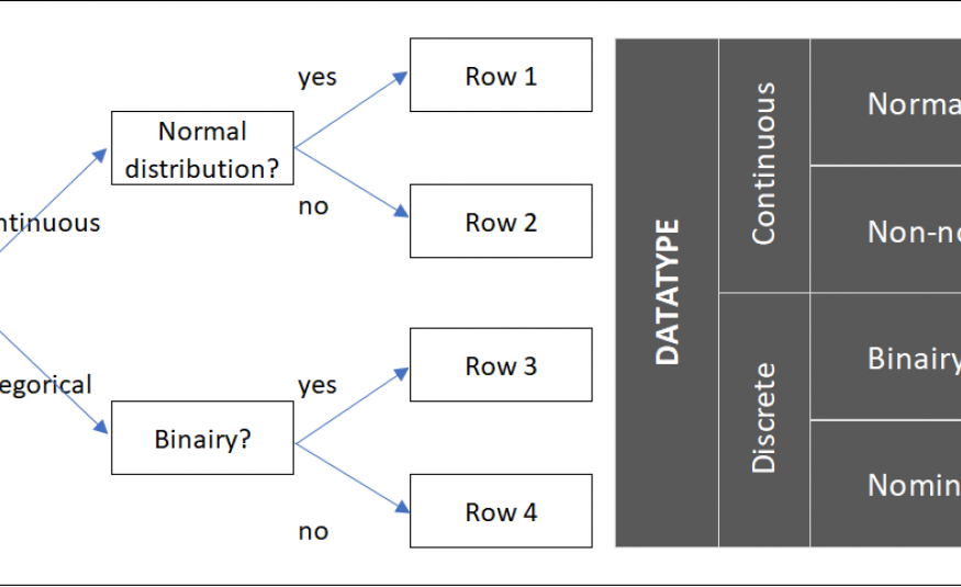
To choose which statistical test you can use in a certain step of the project, you need to know the type of data that is available in the project. The first question we must therefore answer is: WHAT TYPE OF DATA does the project team have available and what are we looking at? We distinguish two different types of data within the Green Belt: continuous data and discrete (categorical) data and each of these two can be divided into two subtypes. Four different data sets are created, shown in Figure 1. The first question included in the figure is whether we are dealing with continuous data or with discrete/categorical data.
Continuous data means that the dataset consists of quantitative data that is measured in a unit and with which you can calculate. Hours, degrees Celsius, centimeters, or even IQ points are all examples of continuous data. They move on a scale that can be divided into units that we can measure.
Discrete/Categorical data is data that cannot be measured on a scale but describes categories. Dividing datasets into groups as good and not good is an example of categories. A second example is the comparison of data from different machines: machine 1, 2, and 3 are three categories.
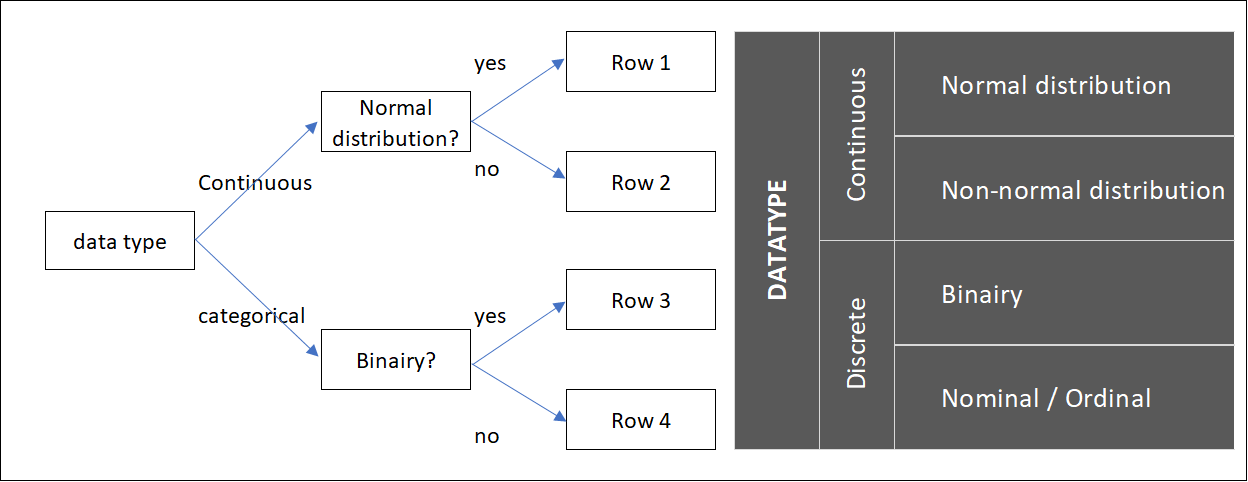
Figure 1: Four types of data
When dealing with continuous data, the following question is important: is the data normally distributed? Or are we dealing with a data set that is not normally distributed?
Whether the data series has a NORMAL DISTRIBUTION or not can be partly determined by the histogram described in Chapter 6. A normal distribution can be recognized when the shape of a histogram looks like that shown in Figure 2. The data then has the following three properties:
- Observations around the mean are most likely,
- The further values are from the mean, the less likely it is to observe those specific values
- Values above and below the mean are equally likely.
The horizontal axis shows the Z-score, and this is the number of standard deviations a data point is removed from the mean. Remember from Chapter 1 that the standard deviation of the data describes the mean deviation of data points from the mean (Appendix 1 describes how to calculate the standard deviation).
A data point with Z = 1 means that the data point is exactly one standard deviation from the mean. Within a normal distribution, 68.2% of the observations (34.1% on the left and 34.1% on the right) are within one standard deviation.
Z=2 means that a data point is two times the standard deviation from the mean, and within a normal distribution, 95.2% of all observations are within two standard deviations.
Finally, the value Z=3 means that a data point is 3x the standard deviation from the mean. With a normal distribution, 99.7% of the data points have a value that is lower than Z=3.
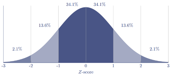
Figure 2: a normal distribution with standard deviations
To test whether a dataset is normally distributed, you can use the Anderson Darling test. The output of this test includes the p-value, a value between 0 and 1. The closer the significance value is to 1, the more "normal" the data set is distributed. Is the significance value <0.05? Then we call the dataset non-normally distributed. We call the data "normally distributed" for all values above 0.05.
A normal distribution, therefore, means that the distribution is symmetrically concentrated around a central value and deviations from this central value become increasingly unlikely the greater the deviation. Figure 3 shows an example where people's intelligence is displayed in a graph. The number of highly intelligent gifted people would be just as great as the number of people with a very low IQ, but the most common IQ of people is in in fact in the middle.

Figure 3: Intelligence of people as a normal distribution
The second type of data is the NON NORMAL DISTRIBUTED DATA. We are again talking about quantitative data with values that go up and down, but in this case, the data is not normally distributed, which means that the deviations are not as predictable as with a normal distribution.
The dataset can have a different type of distribution than the normal distribution, such as the bi-normal, or skewed, as we saw when discussing the histogram in Figure 44 in Chapter 6, or the data is distribution-free, which means that no pattern can be discovered in the current way of representation. An example of distribution-free data is the age of people, see Figure 4. This type of data is also called non-parametric data.
A median age of 50 years in relation to the number of one-year-olds, in this case, does not say anything about the number of 100-year-olds, nor about 5-year-olds.
With distribution-free data, you should look at all data points separately in order to be able to make a statement about significance with any arbitrary factor.
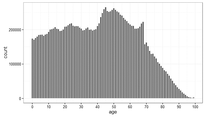
Figure 4: distribution of the age of the Dutch in 2006
We can also split the categorical data into two parts: binary and ordinal data sets. BINARY DATA is not continuous but categorical, and consists of two values: yes/no, male/female, alive/dead. You cannot calculate with these data as with continuous values. You categorize the data points into two groups.
Finally, there are the NOMINAL AND ORDINAL DATASETS. Nominal values are also categorical data, but with more than two categories. One example is a car brand of a test subject's car. A brand is a collective name for a category, of which more than two will occur in a dataset. Nominal values can also include numbers, for instance a telephone number. A telephone number is a number, but you cannot subtract them from each other to make calculations.
Ordinal datasets are categories that cannot be used for mathematical functions like addition and subtraction, but you can order them in a sequence. School reports are an example of this, where we have either numbers (in Europe) or letters (US) which can be put in order and say something about the data set. For instance: an A+ is a better result than a B.
Continue to:
*This article is a copy from the chapter of my book: Six Sigma DMAIC - 8 Simple Steps for Successful Projects
REFERENCE:
Panneman, T., Stemann, D., 2021, Six Sigma DMAIC - 8 Simple Steps for Successful Projects, Ireland: (summary / order this book)