
The standard deviation (Sigma, σ for the population, or S for a sample within the population) of a data series is a measure related to the distribution of the numbers in that series. It is a value that tells you how much on average you deviate from the mean. The smaller the standard deviation (and thus the spread), the better it is. Within six sigma there are two different types of standard deviation. Overall standard deviation (described in Minitab as StdDev(Overall) ) and standard deviation within, which takes subgroups of data into account. This is described as StdDev(within) in Minitab.
Understanding the difference between these two is important to be able to understand the difference between Cp/Cpk and Pk/Ppk in chapter 6, and the difference between the different control charts as part of statistical Process Control in chapter 10.
Let us start with the Standard Deviation (overall), in which we throw all datapoints on one pile and follow the following 4 steps to calculate it:
- Calculate the mean of the data series
- For each number in the series, subtract the mean and square the result.
- Divide the sum of all numbers calculated in step 2 by the number of readings minus 1.
- Take the square root of the result from step 3.
In formula form it looks like this:

Where: S2 = the standard deviation (overall) in the sample, n = the number of values in the series, xi = one of the values in the series, and x̄ = the mean.
A floral example. Suppose we want to calculate the distribution of the number of tulips in a bunch that we can buy at the flower market in Amsterdam. We take 10 bunches of tulips and count the number of tulips for each of those bunches: 9, 2, 5, 4, 12, 7, 8, 11, 9, 3
Step 1 to calculate the standard deviation is to determine the mean of this series:
9+2+5+4+12+7+8+11+9+3/10
= 70/10 = 7
So: x̄ = 7
In step 2, we calculate the difference from the mean for each of the values and square that number (so that it always comes out positive). So:
(9 - 7)2 = (2)2 = 4 (7 - 7)2 = (0)2 = 0
(2 - 7)2 = (-5)2 = 25 (8 - 7)2 = (1)2 = 1
(5 – 7)2 = (-2)2 = 4 (11 - 7)2 = (4)2 = 16
(4 – 7)2 = (-3)2 = 9 (9 - 7)2 = (2)2 = 4
(12 - 7)2 = (5)2 = 25 (3 - 7)2 = (-4)2 = 16
In step 3, we calculate the variance within the series by first adding all the values from step 2 together, and dividing the result by the number of digits -1:
4+25+4+9+25+0+1+16+4+16 = 104
104/(10-1) = 11.556
In step 4, we take the square root of the answer from step 3:
√(11.556) = 3,399
The standard deviation (overall) of the tulip bunches is thus 3.399.
You can, of course, also perform the calculation in Microsoft Excel, Minitab, JMP or SPSS, for example. Figure 97 shows the results of part of the graphical summary of the above example in Minitab. On the right side, we see the values mean and the StdDev (standard deviation) that correspond to the by us calculated values 7 and 3,399.
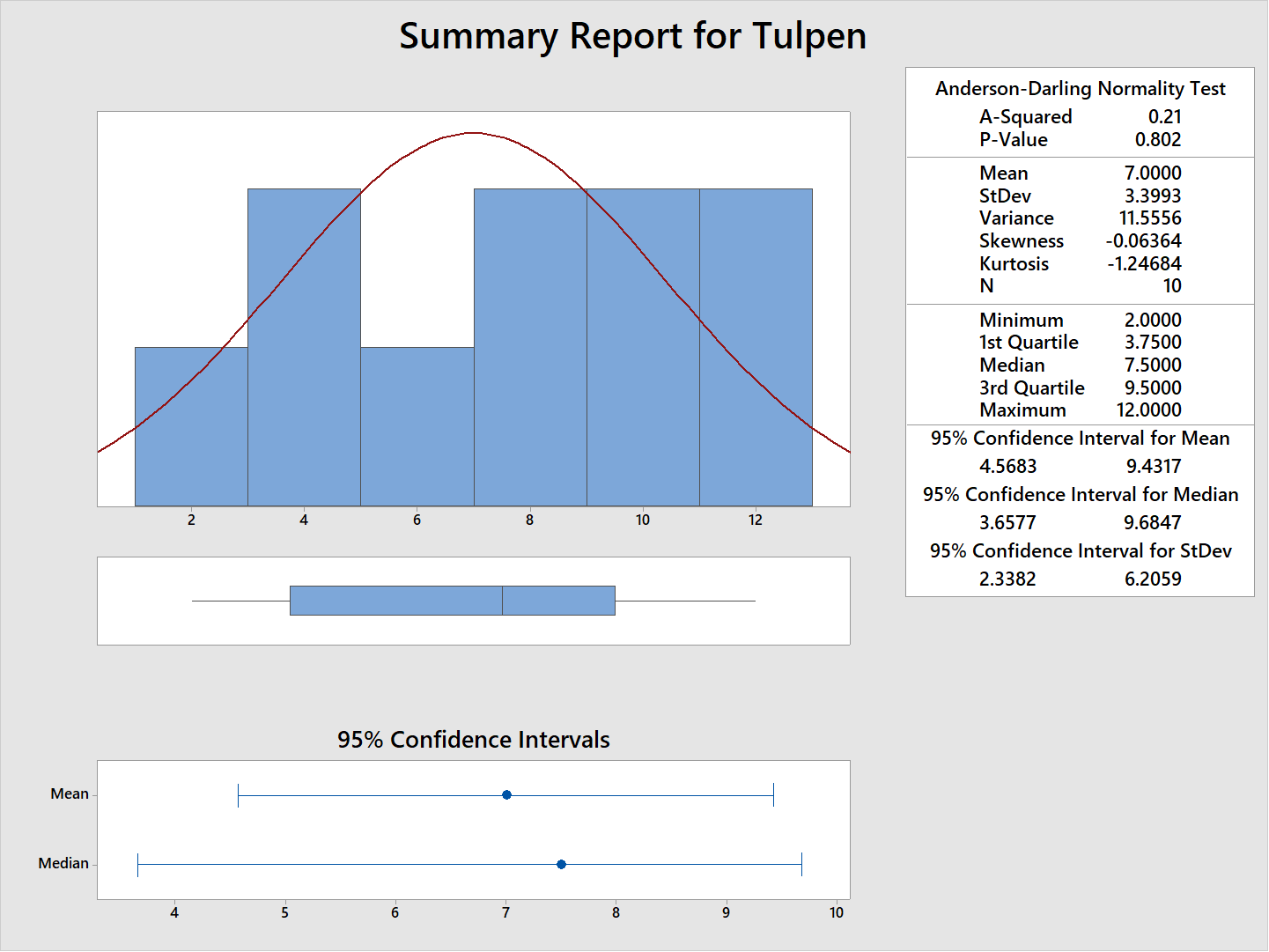
Figure 97: Standard deviation in Tulip example
The Standard Deviation Overall is the easiest one to calculate and can be used in control charts to indicate whether there is common cause variation of special cause variation in the performance. Throwing all datapoints on one pile however can also provide us with an inaccurate picture, for instance when we can buy different types of tulips at the flower market. Size and tulip family can have an impact on how many tulips we find in a bouquet.
This is where the SUBGROUPS come into play and the so-called Standard Deviation Within. In this calculation, we consider that subgroups of datapoints may differ from each other. If we would buy flowers in Amsterdam every day, we would track that the first 10 samples were on Monday and contain common red roses, on Tuesday they contained 10 bouquets of the more expensive Pink Parfait roses and on Wednesday we buy red roses again, etc.
The Standard Deviation (overall) would take all datapoints of the entire month and calculate one number as an output. The Standard Deviation (within) will calculate the standard deviation of each subgroup (the samples collected on the same day) and compare them with each other. Doing this provides us the possibility to capture the common cause variation within each subgroup (in this example different tulips) and visualize the special cause variation between the subgroups.
This is why in terms of control charts (chapter 10) Xbar-S charts are more accurate than the simple I-charts, because common variation is taken out of the dataset by capturing them into subgroups.
Continue to:
Introduction to Six Sigma - Discrete versus Continous Data
*This article is a copy from the chapter of the book: Six Sigma DMAIC - 8 Simple Steps for Successful Projects
REFERENCE:
Panneman, T., Stemann, D., 2021, Six Sigma DMAIC - 8 Simple Steps for Successful Projects, Ireland: (summary / order this book)